COGS 108 - A Structural Characteristic: California Wildfire Damage
Permissions
Place an X in the appropriate bracket below to specify if you would like your group's project to be made available to the public. (Note that student names will be included (but PIDs will be scraped from any groups who include their PIDs).
- [ X ] YES - make available
- [ ] NO - keep private
Names
- Sophie
- Cesar
- Allen
- Ali
- Shahmun
Abstract
Our project examines how the structural characteristics, such as building materials, construction year, and geographical factors contribute to the survival rate of buildings during California Wildfires during the past decade. Motivitated by the growing occurences and the severity of wildfires across the state, we want to see if newer fire-resistant construction methods corroborate with a higher rate of lasting through these events. To further our motive, we combined structural damage assessment data with geospatial data, helping us to visualize and analyze patterns in building survival by region.
Our analyses revelas that both building age and specific structural choices play role in resisting fires and its damage. Specifically, structures built within the last ten years that adhered to building codes, showed a significantly higher survival rate. Additionally, the analysis shows the geographical location is influential, in other words certain regions (northern and central) experiences more intense fire impacts. Overall, our findings highlight the importance of continuous improvements in building codes, adopting fire-resistant material, targeted policy, and understanding the geography accounts for wildfire risk.
Research Question
How do structural characteristics (building materials, age, etc) influence the survival rate of buildings during California wildfires from 2014-2024, and does this relationship vary by geographic region?
Background and Prior Work
Wildfires in California devastate thousands of residents every year causing widespread destruction to home, infrastructure, and ecosystems. With rising global temperatures, prolonged droughts, and increased human activity in fire-prone areas, these wildfires have only escalated. By February of 2025, CAL FIRE had already responded to over 300 wildfires and over 400 structure fires with over 50,000 acres of land burned [1]. This is mostly due to the recent Southern California wildfires which displaced over 100,000 people in the LA metro [2]. As wildfires continue to intensify in the coming years, understanding the vulnerabilities of various types of structures—from single-family homes to commercial districts and historic landmarks—is essential for improving fire-resistant building materials, zoning policies, and emergency response strategies.
One previous work includes a study from the University of California, San Barbara’s Environmental Markets lab which analyzed long-term trends in wildfire damages in California from 1979 to 2018. The study compiled fire perimeter df from CAL FIRE’s Fire and Resource Assessment Program (FRAP) and overlaid it with Wildland Urban Interface (WUI) df to assess the impact of wildfires on structures. The report emphasizes the need for improved fire prevention policies, building codes, and land-use planning to mitigate structural losses in fire-prone regions. The findings align with broader research trends that suggest climate change, increased development in fire-prone areas, and shifting fire seasonality are exacerbating the risks to homes, businesses, and infrastructure [3].
Another previous work is from the Association for Fire Ecology which shows that homes built before 1997 had the lowest survival rate (around 11.5%) while homes built after 1997 had a significantly higher survival rate. The study overall supported fire-resistant construction and wider home separation. For homes built after 2008, after California adopted chapter 7A of the building code, they were even more likely to survive wildfires [4]. In general, chapter 7A of the building code requires for the exterior of a structure to be flame-resistant and ember-resistant during a wildfire[5]. Although previous works done one this matter show that it is not a direct cause and effect of building chacteristics and survival rates, we are interested in analysing the correlation between the two and create more fire-resistant buildings in California. To help further support our question, we must also anaylize the geography of where the building is located, and how prone the area is to fires.
References
- California Department of Forestry and Fire Protection (CAL FIRE). Wildfire Statistics. [Link]
- Inside Climate News. "Los Angeles Fire Victims Seek Therapy After Devastating Wildfires." [Link]
- University of California, Santa Barbara - Environmental Markets Lab. "Wildfire Impact Analysis." [Link]
- Knapp, E. E., Valachovic, Y. S., Quarles, S. L., & Johnson, N. G. (2021). "Housing arrangement and vegetation factors associated with single-family home survival in the 2018 Camp Fire, California." Fire Ecology. [Link]
- Materials and Construction Methods For Exterior Wildfire Exposure.[Link]
Hypothesis
Buildings constructed with fire-resistant materials and built within the last 10 years will have significantly higher survival rates during wildfires compared to older buildings with traditional materials. We predict this because with the advancements of numerous structural innovation technologies and continuous updates in buliding codes/requirements for new builidings, the structural engineering for these buildings to withstand wildfire damage compared to buildings built many years ago should result in a very apparent difference.
Data
Data overview
- Dataset
- Dataset Name: The California Wildfire Data
- Link to the Dataset: https://www.kaggle.com/datasets/vijayveersingh/the-california-wildfire-data/data
- Number of observations: ~100,000
- Number of variables: ~47 (varies by filetype)
The California Wildfire data provides structural damage assessment data for various fire incidents across California. It includes key variables such as DAMAGE, which categorizes the level of destruction, LATITUDE and LONGITUDE for geospatial analysis, and ASSESSEDIMPROVEDVALUE, which reflects the financial impact of fire damage. Other attributes, like INCIDENTNAME and YEARBUILT, can help analyze structural vulnerabilities and trends in wildfire damage over time. The dataset contains two versions (.csv and .geojson) that will be used in conjunction to another for performance reasons and significant file size readings.
The dataset consists of both categorical (e.g., DAMAGE, CITY, STREETNAME) and numerical (e.g., ASSESSEDIMPROVEDVALUE, YEARBUILT) variables, as well as geospatial data in the geometry field. To prepare this dataset for analysis, we need to handle missing values, convert data types where necessary, and remove irrelevant or redundant columns such as OBJECTID and GLOBALID. Additionally, geospatial processing will be required to make full use of location-based trends, and exploratory data analysis (EDA) techniques like visualizing damage levels and geographic clustering will help uncover key insights into wildfire impact patterns.
Column Descriptions (similar conventions for both its .csv and .geojson content)
- OBJECTID: A unique identifier for each record in the dfset.
- DAMAGE: Indicates the level of fire damage to the structure (e.g., "No Damage", "Affected (1-9%)").
- STREETNUMBER: The street number of the impacted structure.
- STREETNAME: The name of the street where the impacted structure is located.
- STREETTYPE: The type of street (e.g., "Road", "Lane").
- STREETSUFFIX: Additional address information, such as apartment or building numbers (if applicable).
- CITY: The city where the impacted structure is located.
- STATE: The state abbreviation (e.g., "CA" for California).
- ZIPCODE: The postal code of the impacted structure.
- CALFIREUNIT: The CAL FIRE unit responsible for the area.
- COUNTY: The county where the impacted structure is located.
- COMMUNITY: The community or neighborhood of the structure.
- INCIDENTNAME: The name of the fire incident that impacted the structure.
- APN: The Assessor’s Parcel Number (APN) of the property.
- ASSESSEDIMPROVEDVALUE: The assessed value of the improved property (e.g., structures, not just land).
- YEARBUILT: The year the structure was built.
- SITEADDRESS: The full address of the property, including city, state, and ZIP code.
- GLOBALID: A globally unique identifier for each record.
- Latitude: The latitude coordinate of the structure’s location.
- Longitude: The longitude coordinate of the structure’s location.
- UTILITYMISCSTRUCTUREDISTANCE: The distance between the main structure and any utility or miscellaneous structures (if recorded).
- FIRENAME: An alternative or secondary name for the fire incident.
- geometry: A geospatial representation of the location in a point format (e.g., "POINT (-13585927.697 4646740.750)").
The dfset reflects the damage sustained by structures across various fire incidents, categorized by damage percentage—ranging from minor damage (1-10%) to complete destruction (50-100%) and collected by field inspectors who evaluate structures impacted by wildland fires.
To clean our dataset, we can apply methods learned in class, such as removing empty columns and rows or filtering out any missing data that is irrelevant to our prediction label. Additionally, exploratory data analysis (EDA) techniques will be useful, including visualizations that highlight the most common damage levels. We can also create figures to identify geographic patterns, assess structural impact, and analyze the distribution of fire incidents across California.
import pandas as pd
import numpy as np
import matplotlib.pyplot as plt
import seaborn as sns

# %pip install geopandas
import geopandas as gpd

import warnings

warnings.filterwarnings('ignore', category=Warning)
After loading our libraries, we must load the dataframe we will use to support our hypothesis.
df = pd.read_csv('../california_wildfire.csv')
df.describe()
| _id | OBJECTID | * Street Number | Zip Code | # Units in Structure (if multi unit) | # of Damaged Outbuildings < 120 SQFT | # of Non Damaged Outbuildings < 120 SQFT | Assessed Improved Value (parcel) | Year Built (parcel) | Latitude | Longitude | x | y | |
|---|---|---|---|---|---|---|---|---|---|---|---|---|---|
| count | 100230.000000 | 100230.000000 | 9.581000e+04 | 47429.000000 | 31184.000000 | 31085.000000 | 31073.00000 | 9.419500e+04 | 69812.000000 | 100230.000000 | 100230.000000 | 1.002300e+05 | 1.002300e+05 |
| mean | 50115.500000 | 50227.779717 | 3.886722e+04 | 46309.699973 | 0.433299 | 0.087566 | 0.12152 | 7.337022e+05 | 1672.283862 | 38.322953 | -121.179297 | -1.348962e+07 | 4.629002e+06 |
| std | 28934.053078 | 29107.678335 | 5.271695e+06 | 47467.653484 | 34.608767 | 0.462729 | 0.52558 | 8.603013e+06 | 708.451814 | 2.019086 | 1.538342 | 1.712474e+05 | 2.825063e+05 |
| min | 1.000000 | 1.000000 | 0.000000e+00 | 0.000000 | 0.000000 | 0.000000 | 0.00000 | 0.000000e+00 | 0.000000 | 32.592548 | -123.774580 | -1.377852e+07 | 3.841346e+06 |
| 25% | 25058.250000 | 25058.250000 | 7.232500e+02 | 0.000000 | 0.000000 | 0.000000 | 0.00000 | 5.937000e+04 | 1944.000000 | 37.350926 | -122.316162 | -1.361617e+07 | 4.488135e+06 |
| 50% | 50115.500000 | 50115.500000 | 4.308500e+03 | 0.000000 | 0.000000 | 0.000000 | 0.00000 | 1.455510e+05 | 1972.000000 | 38.692955 | -121.600277 | -1.353648e+07 | 4.677785e+06 |
| 75% | 75172.750000 | 75172.750000 | 1.000300e+04 | 95667.000000 | 0.000000 | 0.000000 | 0.00000 | 3.109355e+05 | 1987.000000 | 39.763874 | -120.509278 | -1.341503e+07 | 4.831688e+06 |
| max | 100230.000000 | 101221.000000 | 1.410065e+09 | 96311.000000 | 6101.000000 | 40.000000 | 20.00000 | 1.220403e+09 | 2022.000000 | 41.991195 | -116.418163 | -1.295961e+07 | 5.159661e+06 |
After loading our data, we will see the structural characterisitcs we can use to support our hypothesis. This includes damage, year built, etc. We may also begin our Data Cleaning processes such as dropping variables, replacing missing values, and other methods that will help with our analytics.
df.head()
| _id | OBJECTID | * Damage | * Street Number | * Street Name | * Street Type (e.g. road, drive, lane, etc.) | Street Suffix (e.g. apt. 23, blding C) | * City | State | Zip Code | ... | Fire Name (Secondary) | APN (parcel) | Assessed Improved Value (parcel) | Year Built (parcel) | Site Address (parcel) | GLOBALID | Latitude | Longitude | x | y | |
|---|---|---|---|---|---|---|---|---|---|---|---|---|---|---|---|---|---|---|---|---|---|
| 0 | 1 | 1 | No Damage | 8376.0 | Quail Canyon | Road | NaN | Winters | CA | NaN | ... | Quail | 0101090290 | 510000.0 | 1997.0 | 8376 QUAIL CANYON RD VACAVILLE CA 95688 | e1919a06-b4c6-476d-99e5-f0b45b070de8 | 38.474960 | -122.044465 | -1.358593e+07 | 4.646741e+06 |
| 1 | 2 | 2 | Affected (1-9%) | 8402.0 | Quail Canyon | Road | NaN | Winters | CA | NaN | ... | Quail | 0101090270 | 573052.0 | 1980.0 | 8402 QUAIL CANYON RD VACAVILLE CA 95688 | b090eeb6-5b18-421e-9723-af7c9144587c | 38.477442 | -122.043252 | -1.358579e+07 | 4.647094e+06 |
| 2 | 3 | 3 | No Damage | 8430.0 | Quail Canyon | Road | NaN | Winters | CA | NaN | ... | Quail | 0101090310 | 350151.0 | 2004.0 | 8430 QUAIL CANYON RD VACAVILLE CA 95688 | 268da70b-753f-46aa-8fb1-327099337395 | 38.479358 | -122.044585 | -1.358594e+07 | 4.647366e+06 |
| 3 | 4 | 4 | No Damage | 3838.0 | Putah Creek | Road | NaN | Winters | CA | NaN | ... | Quail | 0103010240 | 134880.0 | 1981.0 | 3838 PUTAH CREEK RD WINTERS CA 95694 | 64d4a278-5ee9-414a-8bf4-247c5b5c60f9 | 38.487313 | -122.015115 | -1.358266e+07 | 4.648497e+06 |
| 4 | 5 | 5 | No Damage | 3830.0 | Putah Creek | Road | NaN | Winters | CA | NaN | ... | Quail | 0103010220 | 346648.0 | 1980.0 | 3830 PUTAH CREEK RD WINTERS CA 95694 | 1b44b214-01fd-4f06-b764-eb42a1ec93d7 | 38.485636 | -122.016122 | -1.358277e+07 | 4.648259e+06 |
5 rows × 47 columns
print(df.columns)
print(df.shape)
Index(['_id', 'OBJECTID', '* Damage', '* Street Number', '* Street Name',
'* Street Type (e.g. road, drive, lane, etc.)',
'Street Suffix (e.g. apt. 23, blding C)', '* City', 'State', 'Zip Code',
'* CAL FIRE Unit', 'County', 'Community', 'Battalion',
'* Incident Name', 'Incident Number (e.g. CAAEU 123456)',
'Incident Start Date', 'Hazard Type',
'If Affected 1-9% - Where did fire start?',
'If Affected 1-9% - What started fire?',
'Structure Defense Actions Taken', '* Structure Type',
'Structure Category', '# Units in Structure (if multi unit)',
'# of Damaged Outbuildings < 120 SQFT',
'# of Non Damaged Outbuildings < 120 SQFT', '* Roof Construction',
'* Eaves', '* Vent Screen', '* Exterior Siding', '* Window Pane',
'* Deck/Porch On Grade', '* Deck/Porch Elevated',
'* Patio Cover/Carport Attached to Structure',
'* Fence Attached to Structure', 'Distance - Propane Tank to Structure',
'Distance - Residence to Utility/Misc Structure > 120 SQFT',
'Fire Name (Secondary)', 'APN (parcel)',
'Assessed Improved Value (parcel)', 'Year Built (parcel)',
'Site Address (parcel)', 'GLOBALID', 'Latitude', 'Longitude', 'x', 'y'],
dtype='object')
(100230, 47)
df = df.drop(['OBJECTID',
              '_id',
              'Street Suffix (e.g. apt. 23, blding C)',
              'State',
              'Zip Code',
              'Community',
              'Battalion',
              'Incident Number (e.g. CAAEU 123456)',
              'Hazard Type',
              'Fire Name (Secondary)',
              'Distance - Residence to Utility/Misc Structure > 120 SQFT',
              'APN (parcel)',
              'Distance - Propane Tank to Structure',
              'GLOBALID',
              'Site Address (parcel)',
              '# Units in Structure (if multi unit)',
              '* Structure Type',
              '* Fence Attached to Structure',
              'x',
              'y',
              '* City',
              '* Incident Name',
              'If Affected 1-9% - Where did fire start?',
              'If Affected 1-9% - What started fire?',
              '# of Damaged Outbuildings < 120 SQFT',
              '# of Non Damaged Outbuildings < 120 SQFT'
             ], axis=1)
Dropped non-informative data including parcel numbers to ids and minor outbuilding damage to focus on structural materials and proximity to vegetation
df['Structure Defense Actions Taken'] = df['Structure Defense Actions Taken'].fillna('None')
df = df.dropna()
print(df.isnull().values.any())
df = df.drop_duplicates(keep='first')
print(df.duplicated().sum())
df.head()
False
0
| * Damage | * Street Number | * Street Name | * Street Type (e.g. road, drive, lane, etc.) | * CAL FIRE Unit | County | Incident Start Date | Structure Defense Actions Taken | Structure Category | * Roof Construction | ... | * Vent Screen | * Exterior Siding | * Window Pane | * Deck/Porch On Grade | * Deck/Porch Elevated | * Patio Cover/Carport Attached to Structure | Assessed Improved Value (parcel) | Year Built (parcel) | Latitude | Longitude | |
|---|---|---|---|---|---|---|---|---|---|---|---|---|---|---|---|---|---|---|---|---|---|
| 0 | No Damage | 8376.0 | Quail Canyon | Road | LNU | Solano | 6/6/2020 12:00:00 AM | None | Single Residence | Asphalt | ... | Mesh Screen <= 1/8"" | Wood | Single Pane | Wood | Wood | No Patio Cover/Carport | 510000.0 | 1997.0 | 38.474960 | -122.044465 |
| 1 | Affected (1-9%) | 8402.0 | Quail Canyon | Road | LNU | Solano | 6/6/2020 12:00:00 AM | Hand Crew Fuel Break | Single Residence | Asphalt | ... | Mesh Screen <= 1/8"" | Wood | Multi Pane | Masonry/Concrete | No Deck/Porch | No Patio Cover/Carport | 573052.0 | 1980.0 | 38.477442 | -122.043252 |
| 2 | No Damage | 8430.0 | Quail Canyon | Road | LNU | Solano | 6/6/2020 12:00:00 AM | None | Single Residence | Asphalt | ... | Mesh Screen > 1/8"" | Wood | Single Pane | No Deck/Porch | No Deck/Porch | No Patio Cover/Carport | 350151.0 | 2004.0 | 38.479358 | -122.044585 |
| 3 | No Damage | 3838.0 | Putah Creek | Road | LNU | Solano | 6/6/2020 12:00:00 AM | None | Single Residence | Asphalt | ... | Mesh Screen > 1/8"" | Wood | Single Pane | No Deck/Porch | No Deck/Porch | Combustible | 134880.0 | 1981.0 | 38.487313 | -122.015115 |
| 4 | No Damage | 3830.0 | Putah Creek | Road | LNU | Solano | 6/6/2020 12:00:00 AM | None | Single Residence | Tile | ... | Mesh Screen > 1/8"" | Wood | Multi Pane | Wood | Wood | Combustible | 346648.0 | 1980.0 | 38.485636 | -122.016122 |
5 rows × 21 columns
geo_df = gpd.read_file('../geo_california_wildfire.geojson')
df.describe()
| * Street Number | Assessed Improved Value (parcel) | Year Built (parcel) | Latitude | Longitude | |
|---|---|---|---|---|---|
| count | 5.914000e+04 | 5.914000e+04 | 59140.000000 | 59140.000000 | 59140.000000 |
| mean | 5.406353e+04 | 8.358812e+05 | 1676.543236 | 38.189823 | -121.077250 |
| std | 6.709125e+06 | 1.023007e+07 | 703.690732 | 2.120131 | 1.551404 |
| min | 0.000000e+00 | 0.000000e+00 | 0.000000 | 32.592548 | -123.683036 |
| 25% | 9.590000e+02 | 6.000000e+04 | 1945.000000 | 37.138162 | -122.143732 |
| 50% | 5.110000e+03 | 1.445120e+05 | 1971.000000 | 38.665997 | -121.598170 |
| 75% | 9.865000e+03 | 3.111675e+05 | 1986.000000 | 39.763468 | -119.968393 |
| max | 1.410065e+09 | 1.220403e+09 | 2022.000000 | 41.935088 | -116.623886 |
print(geo_df.columns)
print(geo_df.shape)
Index(['OBJECTID', 'DAMAGE', 'STREETNUMBER', 'STREETNAME', 'STREETTYPE',
       'STREETSUFFIX', 'CITY', 'STATE', 'ZIPCODE', 'CALFIREUNIT', 'COUNTY',
       'COMMUNITY', 'BATTALION', 'INCIDENTNAME', 'INCIDENTNUM',
       'INCIDENTSTARTDATE', 'HAZARDTYPE', 'WHEREFIRESTARTEDONSTRUCTURE',
       'WHATDIDFIRESTARTFROM', 'DEFENSIVEACTIONS', 'STRUCTURETYPE',
       'STRUCTURECATEGORY', 'NUMBEROFUNITPERSTRUCTURE',
       'NOOUTBUILDINGSDAMAGED', 'NOOUTBUILDINGSNOTDAMAGED', 'ROOFCONSTRUCTION',
       'EAVES', 'VENTSCREEN', 'EXTERIORSIDING', 'WINDOWPANE',
       'DECKPORCHONGRADE', 'DECKPORCHELEVATED', 'PATIOCOVERCARPORT',
       'FENCEATTACHEDTOSTRUCTURE', 'PROPANETANKDISTANCE',
       'UTILITYMISCSTRUCTUREDISTANCE', 'FIRENAME', 'APN',
       'ASSESSEDIMPROVEDVALUE', 'YEARBUILT', 'SITEADDRESS', 'GLOBALID',
       'Latitude', 'Longitude', 'geometry'],
      dtype='object')
(100230, 45)
geo_df = geo_df.dropna()
geo_df["YEARBUILT"] = pd.to_numeric(geo_df["YEARBUILT"]) # Convert numeric
geo_df = geo_df.drop(columns=["OBJECTID",
                              "STATE",
                              "ZIPCODE",
                              "COMMUNITY",
                              "BATTALION",
                              "INCIDENTNUM",
                              "HAZARDTYPE",
                              "FIRENAME",
                              "APN",
                              "SITEADDRESS",
                              "GLOBALID",
                              "PROPANETANKDISTANCE",
                              "UTILITYMISCSTRUCTUREDISTANCE",
                              "NOOUTBUILDINGSDAMAGED",
                              "NOOUTBUILDINGSNOTDAMAGED",
                              "NUMBEROFUNITPERSTRUCTURE"]
                              , axis=1) # Similar to .csv
geo_df.head()
| DAMAGE | STREETNUMBER | STREETNAME | STREETTYPE | STREETSUFFIX | CITY | CALFIREUNIT | COUNTY | INCIDENTNAME | INCIDENTSTARTDATE | ... | WINDOWPANE | DECKPORCHONGRADE | DECKPORCHELEVATED | PATIOCOVERCARPORT | FENCEATTACHEDTOSTRUCTURE | ASSESSEDIMPROVEDVALUE | YEARBUILT | Latitude | Longitude | geometry | |
|---|---|---|---|---|---|---|---|---|---|---|---|---|---|---|---|---|---|---|---|---|---|
| 74513 | Destroyed (>50%) | 4300.0 | High | Road | Montague | SKU | Siskiyou | High | Fri, 24 May 2019 00:00:00 GMT | ... | Single Pane | Wood | No Deck/Porch | No Patio Cover/Carport | No Fence | 15000.0 | 1977.0 | 41.669654 | -122.544020 | POINT (-13641537.957 5111622.953) | |
| 74514 | Destroyed (>50%) | 2980.0 | 16 State Highway | None | Ramsey | LNU | Yolo | Sand | Sat, 08 Jun 2019 00:00:00 GMT | ... | No Windows | No Deck/Porch | No Deck/Porch | No Patio Cover/Carport | No Fence | 31486.0 | 1923.0 | 38.894719 | -122.249752 | POINT (-13608780.135 4706602.181) | |
| 74515 | Destroyed (>50%) | 2559.0 | Rumsey Canyon | Road | Rumsey | LNU | Yolo | Sand | Sat, 08 Jun 2019 00:00:00 GMT | ... | Single Pane | No Deck/Porch | No Deck/Porch | No Patio Cover/Carport | No Fence | 242760.0 | 1975.0 | 38.902134 | -122.246907 | POINT (-13608463.4 4707662.808) | |
| 74516 | Destroyed (>50%) | 2756.0 | Rumsey Canyon | Road | Rumsey | LNU | Yolo | Sand | Sat, 08 Jun 2019 00:00:00 GMT | ... | Unknown | No Deck/Porch | No Deck/Porch | Non Combustible | No Fence | 46552.0 | 0.0 | 38.900564 | -122.249926 | POINT (-13608799.488 4707438.274) | |
| 74517 | Destroyed (>50%) | 2756.0 | Rumsey Canyon | Road | Rumsey | LNU | Yolo | Sand | Sat, 08 Jun 2019 00:00:00 GMT | ... | Unknown | No Deck/Porch | No Deck/Porch | Unknown | No Fence | 46552.0 | 0.0 | 38.900753 | -122.250288 | POINT (-13608839.798 4707465.236) |
5 rows × 29 columns
Section 1 of EDA - Fire Analysis
In this section we will be looking at our dataset to understand what information we can gather from it. We will be looking at the damages type counts, as well as the number of fires over a period of time, if there are relations to time of year and fire incidents, and possibly more that we will get into during our EDA (.csv).
damages = df['* Damage'].value_counts()
sns.barplot(x=damages.index, y=damages.values, color="orange")
plt.xlabel('Damage Types')
plt.ylabel('Counts')
plt.title('Bar Plot of Damage Type Counts')
plt.xticks(rotation=45)
plt.show()

From this plot we can see that the most common types of damage caused by fires in the state are result in mainly more than 50% destroyed, 0% destroyed, and barely affected (1-9%). We can use this information to compare what conditions resulted in buildings and other structures being more than half desotryed compared to the buildings that barely suffered any to no damage.
df['Incident Start Date'] = pd.to_datetime(df['Incident Start Date'], errors='coerce')

# Drop rows with invalid dates
df = df.dropna(subset=['Incident Start Date'])

# Extract the year from 'Incident Start Date'
df['Year'] = df['Incident Start Date'].dt.year
df['Year'].value_counts()

incident_counts_by_year = df['Year'].value_counts().sort_index()

sns.lineplot(x=incident_counts_by_year.index, y=incident_counts_by_year.values)
plt.xlabel('Year')
plt.ylabel('Count')
plt.title('Count Over Time')
plt.xticks(rotation=45)  # Rotate x-axis labels if needed
plt.show()

From our lineplot, we can see that the number of fire incidents over the years has fluctuated from low to high, which is interesting to see from an outside view. There is a number of questions we would like to ask here, as to why the data is shaped liked this. Were there contributing factors occuring in California during these peak periods? Maybe the way we cleaned our data caused the graph to shape itself such as this? These are questions we can hopefully answer with more research surrounding those time periods as well as analyzing how we cleaned our dataset to make sure we account for such things that would affect our research.
df['Month'] = df['Incident Start Date'].dt.month_name()
df['Month'].value_counts()

incident_counts_by_month = df.groupby('Month').size().reset_index(name='count')
month_order = ['January', 'February', 'March', 'April', 'May', 'June', 'July', 'August', 'September', 'October', 'November', 'December']
incident_counts_by_month['Month'] = pd.Categorical(incident_counts_by_month['Month'], categories=month_order, ordered=True)
incident_counts_by_month = incident_counts_by_month.sort_values('Month')

sns.barplot(x='Month', y='count', data=incident_counts_by_month, color="green")
plt.xlabel('Month')
plt.ylabel('Count')
plt.title('Fire Count per Month')
plt.xticks(rotation=45)  # Rotate x-axis labels if needed
plt.show()

The plot above shows us the count of fires over the period 2014-2024 that have happened each month, where we look at any pattern in time of year that relates to the number of fires. We can see that the most fires occur in the later half of the year between the months of May/June and December/January, with peaks in August to November range. We know that the seasons in this time of year are summer, fall, and winter, and knowing the type of climate that California has which is usually dry and hot, it is not unreasonable to have such data. It would definitely be intersting to research why there is such a big peak in November especially, because there could be a big number of reasons as to why this peaks here, but we would have to analyze and do much research to find out why this disparity exists.
Section 2 of EDA - Structural Analysis
In this part of our EDA analysis, we will be covering more about the structural information of the buildings in our dataset. We will cover survival stats from builiding materials, survival from building age, survival status by Geographic Region, and more we will get into during our EDA.
current_year = 2025
Year_Built = df[df['Year Built (parcel)'] > 100]
Year_Built['Year_Built'] = Year_Built['Year Built (parcel)']
Year_Built_value_counts = current_year - Year_Built['Year_Built']

plt.figure(figsize=(10,6))
sns.histplot(Year_Built_value_counts, kde=True, bins=100)
plt.title("Distribution of Building Age")
plt.xlabel("Building Age (Years)")
plt.ylabel("Count")
plt.xlim(0, 300)
plt.show()

From our histogram we can see the overall dispersion of the ages of our buildings in our dataset and the overall line or curve that represents our slope of having less buildings of older age. As one would expect, the most buildings in this dataset would be included from our time period which includes about 50 years ago during the 1900s which would be when America was expanding and innovating to now where we still do expand and build however we have slowed down since almost everything has become usurped especially the land. With the building ages taken into account for future reference we can use this to see if the building age affects the survival rate of buildings.
Year_Built['Roof'] = Year_Built['* Roof Construction'].replace(r'^\s*$', None, regex=True)
Year_Built = Year_Built.dropna(subset=['Roof'])

Year_Built['Roof'].value_counts()

plt.figure(figsize=(10,6))
sns.countplot(x='Roof', data=Year_Built,
              order=Year_Built['Roof'].value_counts().index,
              color="teal")
plt.title("Distribution of Building Materials")
plt.xlabel("Building Material")
plt.ylabel("Count")
plt.xticks(rotation=45)
plt.show()

From our barplot we can see that the most common type of material used for these buildings is Asphalt, followed by metal, and then Tile. We can see that we have some lables that are not descriptive or provide any information such as unknown and other, but we keep them there just to represent fire incidents that did occur but ones where we do not have all the information available. We can use the information in this graph to potentially aid us in further analysis as to asking if building materials positively or negatively affect the damage suffered by fire incidents.
plt.figure(figsize=(10,6))
sns.countplot(x='Roof', hue='* Damage', data=Year_Built,
              order=Year_Built['Roof'].value_counts().index)
plt.title("Damage Type suffered for each Building Material")
plt.xlabel("Building Material")
plt.ylabel("Count")
plt.xticks(rotation=45)
plt.show()

This graph gives us a representation of how each building material did with its fire damage, where we split our fire damages into destroyed, major, minor, affected, etc. We can see how the most common material was also the most destroyed, which we can see correlates because of the sheer amount of times it is used by buildiers. However we do see some intersting resutls especially in the unknown section, where the buildings more often than being destroyed actually suffer no damages to the building itself. It would be very useful and impactful if we would find out what this unknown material was as it could not only aid in our research, but help save more buildings from being destroyed and potentially even saving more lives.
damage_counts = Year_Built.groupby('Year_Built')['* Damage'].value_counts().unstack()
plt.figure(figsize=(12, 6))
damage_counts.plot(kind='line', figsize=(12, 6), marker='o')
plt.xlabel('Year Built')
plt.ylabel('Count of Damage Types')
plt.title('Damage Types Over the Years')
plt.legend(title="Damage Type")
plt.show()
<Figure size 1200x600 with 0 Axes>

From this graph that looks at the relationship between type of damage versus building age, we can see a few things that could be important to our findings. One we see that the number of destroyed buildings has increased, which one may think would lead to our hypothesis being wrong about how advances in fire prevention technology and strucutral engineering could lead to significant reduction in fire damage severity, we can also take a look at the other kind of fire damages. We see that what has also increased throughout the years was the number of fires that caused no damage to the structure, as well as fires with affected or minor fire damage. This means that although we have had more buildings be destroyed in fires, we have also have more buildings being saved from being destroyed or greatly damaged which still supports our hypothesis and what we want to prove. There is a drop off though towards the end of our graph, which we can attribute to less fire reportings in recent years, which could be from good fire prevention practices and such.
df2 = df

df2_filtered = df2[['Year Built (parcel)', '* Damage']].dropna()

df2_filtered.columns = ['Year Built', 'Damage']

df2_filtered['Year Built'] = df2_filtered['Year Built'].astype(int)

df2_filtered['Decade Built'] = (df2_filtered['Year Built'] // 10) * 10

# Filter after 1870

df2_filtered_1870 = df2_filtered[df2_filtered['Decade Built'] >= 1870]

houses_per_decade = df2_filtered_1870.groupby('Decade Built').size()

damage_distribution = df2_filtered_1870.groupby(['Decade Built', 'Damage']).size().unstack(fill_value=0)

fraction_damage = damage_distribution.div(houses_per_decade, axis=0)

custom_colors = ['#e6194B',  '#3cb44b',  '#ffe119',  '#4363d8', '#f58231', '#911eb4']

fraction_damage.plot(kind='bar', stacked=True, figsize=(12, 6), color=custom_colors)

plt.title('Fraction of Damage Types per Decade Built (1870 and Onwards)')
plt.xlabel('Decade Built')
plt.ylabel('Ratio of Houses')
plt.legend(title='Damage Type')
plt.xticks(rotation=45)
plt.grid(axis='y', linestyle='--', alpha=0.7)
plt.show()

The graph displays the proportion of different damage types for houses built in each decade from 1870 onwards. Each house is categorized into a decade based on its construction year, and the total number of houses in each decade. The ratio of houses per damage type per decade are then organized and stacked in a bar graph. The stacked bar chart visually represents the damage type proportions, showing how the likelihood of different damage levels varies by construction era. Distinct colors differentiate damage types, allowing for an easy comparison across decades. This visualization highlights trends in structural resilience over time, revealing newer houses tend to suffer less damage.
Section 3 of EDA - Geospatial Analysis
Data analysis using the same dataset through its .geojson contents
import folium
from folium.plugins import HeatMap
m = folium.Map(location=[37.5, -119.5], zoom_start=6)
gradient = {
0.2: "yellow",
0.5: "orange",
0.8: "red",
1.0: "#800000"
}
heat_data = geo_df[["Latitude", "Longitude"]].dropna().values.tolist()
HeatMap(heat_data, radius=10, gradient=gradient).add_to(m)
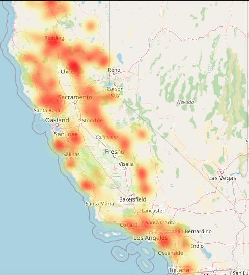
# static image attached since heatmap cannot be rendered on GitHub
<folium.plugins.heat_map.HeatMap at 0x17880ef10>
The above heatmap highlights areas in California that have been most impacted by wildfires, with the most intense activity concentrated in the northern and central parts of the state. The northern regions stand out as major wildfire hotspots due to historical fire patterns. Some insights to dry climate and dense vegetation are valid variables to consider as there are notable clusters/proximity of fire activity from major cities with high human populace that could also contribute to a flammable ecosystem.
Data Analysis and Results
Identify the significant factors that contribute to fire damage severity
from sklearn.model_selection import train_test_split
from sklearn.ensemble import RandomForestClassifier
from sklearn.preprocessing import LabelEncoder
from sklearn.metrics import accuracy_score, classification_report, confusion_matrix
# Random Forest Model
# Create feature set
features = ['Building Age', '* Roof Construction', '* Eaves', '* Vent Screen',
            '* Exterior Siding', '* Window Pane', '* Deck/Porch On Grade',
            '* Deck/Porch Elevated', '* Patio Cover/Carport Attached to Structure',
            'Assessed Improved Value (parcel)', 'Latitude', 'Longitude']
target = '* Damage'
The Random Forest Classifer was fitting because it handles non-linearity relationships and categorical data for classification.
# Preprocess data
df = df[df['Year Built (parcel)'] > 0]
df['Building Age'] = 2025 - df['Year Built (parcel)'] # Using present year as a reference
df_model = df[features + [target]].dropna()

le = LabelEncoder() # Convert to numerical values for modeling
categorical_features = ['* Roof Construction', '* Eaves', '* Vent Screen', '* Exterior Siding', '* Window Pane',
                        '* Deck/Porch On Grade', '* Deck/Porch Elevated', '* Patio Cover/Carport Attached to Structure']
for feature in categorical_features:
    df_model[feature] = le.fit_transform(df_model[feature])

df_model[target] = le.fit_transform(df_model[target])
X = df_model[features]
y = df_model[target]
X_train, X_test, y_train, y_test = train_test_split(X, y, test_size=0.2, random_state=42)

rf_model = RandomForestClassifier(n_estimators=100, random_state=42)
rf_model.fit(X_train, y_train)
y_pred = rf_model.predict(X_test)

accuracy = accuracy_score(y_test, y_pred)
print(classification_report(y_test, y_pred))
              precision    recall  f1-score   support

           0       0.46      0.18      0.26       408
           1       0.94      0.96      0.95      6168
           2       0.73      0.42      0.54        26
           3       0.25      0.05      0.09        56
           4       0.16      0.04      0.06       100
           5       0.90      0.97      0.93      3301

    accuracy                           0.92     10059
   macro avg       0.57      0.44      0.47     10059
weighted avg       0.90      0.92      0.90     10059
Report shows severity from fire damage in multiple sections. Although the accuracy was 92%, performance varies across the different levels of fire damage given from 0-5. The F1-score also indicates this imbalance in consistency so the model is flawed when assesing less common damage types.
sns.heatmap(confusion_matrix(y_test, y_pred), annot=True, fmt='d', cmap='Blues')
plt.xlabel('Predicted')
plt.ylabel('Actual')
plt.title('Confusion Matrix')
plt.show()

The model performs better for classes 1 (minor damage) and 5 (completely destroyed) but struggles with the rarer classes and often misclassifying them.
feature_importance = rf_model.feature_importances_
feature_names = X.columns

plt.figure(figsize=(8,6))
sns.barplot(x=feature_importance, y=feature_names, color='#042E4C')
plt.xlabel('Feature Importance')
plt.ylabel('Feature')
plt.title('Random Forest Feature Importance')
plt.show()

The chart highlights fire damage severity, with exterior siding (outermost protection of a building), latitude, and longitude being the most impactful. Exterior siding was interesting and transparent with how outside walls are the first material to be in contact to flames. Next, the chart has flaws. Certain variables like latitude and longitude are ranked as one of the highest but their direct impact on fire damage may be questionable without additional context such as vegetation or climate. Location would not be enough to translate to a claim or to disprove one. Prior to the previous data, other factors may have high importance due to correlation with fire resistance. The model, however, doesn’t account for this and imbalancing of the damage severity should be addressed noting the reliability and bias of the model. Tuning hyperparameters could help but other factors to consider is the compatibility of the dataset in conjunction to the proposed hypothesis which might not perfectly align with what was gathered. As aforementioned, feature importance helps the interpretability of specific factors but correlation does not confirm causation.
Ethics & Privacy
- Ethical concerns raised for our dataset could pertain to mainly bias concerning rating of structural damage and possibly senstive geospatial property where information should not be leaked.
- Mitigation strategy for confidential locations should be addressed such as anonymizing exact location df to protect restricted property information or property owners.
- There could also pertain a rating bias when quantifying the damage score of how the damaged the structure is depending on the observer who recorded it (ex. somewhat damaged vs slightly damaged).
- Sampling and socioeconomic biases can be considered with how inaccessible locations are not reported or collected and damage assements might not address the difference/disparity in the quality of a structure due to financial or external situations in the area.
- Setting out to detect biases before/during/after communicating our analysis might not be as simple as df collection as it's already created and we can't garner new df with a standarized protocol to rank all inspected structural damage so we'll address the limitation of the df collection and document known biases as a clear communication to our project.
- For any upcoming concerns that might appear during the before/in-progress/after of the project, we will immediately communicate and resolve any concernable flags that will pertain to the ethics checklist such as df security to unintended use of the project's results.
Discussion and Conclusion
Our research and work on our data based aimed to answer our question about: "How do structural characteristics (building materials, age, etc) influence the survival rate of buildings during California wildfires from 2014-2024, and does this relationship vary by geographic region?". Based on our background research and such we hypothesized that buildings built more recently have better survival rates over buildings built more far off, as well as looking at the geographical location that could come into play as a variable.
Our findings seem to be sort of consistent with the prior study we talked about in our background section, from the University of California Santa Barbara. The report emphasizes the need for improved fire prevention policies, building codes, and land-use planning to mitigate structural losses in fire-prone regions. We can see from our EDA on structural analysis and geospatial analysis, was that structures that were older in age were more likely to result in being desotryed rather than only taking minor or affected damage. We can see a small trend in our data that indicates possibly there was a change in how buildings were built and how fire prevention measures were taken because we did see more buildings taking signifcantly less damage all though the number of fires went up including the amount of destroyed buildings. The findings from the UC Santa Barbara's report also suggested that climate change, increased development in fire-prone areas, and shifting fire seasonality are exacerbating the risks to homes, businesses, and infrastructure. This is also shown in our data because the number of fires occuring every year seemed to grow as well over time, which as seen could be attirbuted to a number of factors including global warming and the expansion of real estate into areas that are more prone to fires.
While our analysis provided valuable insights, it was limited by many factors such as missing values in our dataset, relatively small set of data to work with, missing valuable data like distance to vegetation and topography. You can see this especially affects the effectiveness of our model in predicting fire damage based on our features. Also there seems to be some inconsistencies in our dataset, which can be seen in our number of incidents over time plot where there was a huge dip in the number of fires during a small period and then shot right back up which seems strange but could possibly be adressed with research about certain events that occured that year. Future work could address these limitations by making sure our dataset comes frmo reliable sources that provides the information we look for that we lacked in this research. Possibly cleaning the dataset better to perhaps not remove any important data we could have used could be a good step to take next time since even working with the dataset before cleaning a lot of the columns had NaN values in each which made it difficult to see what rows and columns to keep for our EDA. Choosing a better dataset with less NaN values overall would also benefit us as well in the future which will be good for us to learn and effectively do.
These findings could be really usefull for future buyers in the market for realestate or for everyday people looking for their next home. It can really benefit them in their decision making when choosing where and when to buy a home or piece of property, by avoiding areas that have more probability of suffering severe damage to structures as well as being able to make safe precautions during those times of years fires are more likely to occur. This can also be said to construction companies who are building these properties, since we also compared the type of materials used in these structures and how they usually held up. Seeing what materials were more effective like Asphalt cnan help companies make better decisions about material usage in order to prevent less structural damage from fires in the long run. By understanding how different variables affect the structural integrity of buildings during fires, we can help numerous groups who all benefit from one another, creating a safer environment for all and could potentially in the long run save a lot of people from losing homes and memories such as we saw in recent events during the fires all over California in 2025.
Future research could explore different variables and datasets to build on our findings. For example, rising temperatures in the region from global warming and other sources of climate change could defintiely add to our geospatial analysis and how different regions are more or less likely to experience varying fire damage. The type of geography of the region also has a lot to do with how fires occur, especially since woodland areas like national parks or forests are of course more likely to suffer a lot more damage due to the nature of resources located there. Additionally, investigating fire science and precautions/policies taken to preventing such things could provide deeper insights into how new technology in recently built buildings can lower the damage taken by structures in instances of fires. We are sure that there will be more data out there or future data to allow us to investigate further into these topics in order to give people a more accurate prediction about which areas and buildings are less likely to be fully destroyed in fires and which ones are more likely to be destoryed.
Team Contributions
- Allen Vu
- Created ethics and privacy section, created the EDA analysis (geospatial analysis), data analysis and programming.
- Worked on slides.
- Cesar Perez
- Created research question, created hypothesis, created the EDA analysis, data analysis and programming.
- Worked on cleaning the dataset.
- Sophie Smith
- Helped organize the group, write team expectations, project timeline, and helped find the dataset.
- Wrote the final report, created the slide presentation, and wrote abstract.
- Ali
- Worked on the data section (Q1/Q2), fixed issues with data relevance in the description/hypothesis sections.
- Editied the video
- Shahmun Jafri
- Created the script for the final video, editied the video, background and prior work, created one EDA visual.
- Helped find the dataset